3.7. MULTICI: Generate matrix of averaged read density
The MULTICI generates a matrix file that describes the averaged read density in specified BED site:
dir=parse2wigdir+
gt=genometable.hg19.txt
drompa+ MULTICI \
-i $dir/H3K4me3.100.bw,$dir/Input.100.bw,H3K4me3 \
-i $dir/H3K27me3.100.bw,$dir/Input.100.bw,H3K27me3 \
-i $dir/H3K36me3.100.bw,$dir/Input.100.bw,H3K36me3 \
-o drompa --gt $gt --bed H3K4me3.bed
The output file (drompa.MULTICI.averaged.ChIPread.tsv) is a tab-delimited TSV file that contains the averaged ChIP-read intensity per bin size for each BED site like this:
$ head drompa.MULTICI.averaged.ChIPread.tsv
        H3K4me3 H3K27me3        H3K36me3
chr1-137600-138199      38.5659 0       3.15773
chr1-138400-139599      30.6127 1.21359 3.48057
chr1-713000-715499      60.1785 1.05242 1.16351
chr1-761200-761499      21.2679 0       5.60837
chr1-761900-763299      69.3009 0.57135 0.947986
chr1-839300-840799      38.307  1.33495 0.7842
chr1-858900-859099      26.1827 13.0429 0
chr1-859300-861299      48.3319 8.51783 0.29999
chr1-875800-876399      48.9127 14.4279 1.93347
3.7.1. Output ChIP/Input enrichment
Add --stype 1 to generate averaged ChIP/Input enrichment table:
dir=parse2wigdir+
gt=genometable.hg19.txt
drompa+ MULTICI \
-i $dir/H3K4me3.100.bw,$dir/Input.100.bw,H3K4me3 \
-i $dir/H3K27me3.100.bw,$dir/Input.100.bw,H3K27me3 \
-i $dir/H3K36me3.100.bw,$dir/Input.100.bw,H3K36me3 \
-o drompa --gt $gt --bed H3K4me3.bed --stype 1
then drompa.MULTICI.averaged.Enrichment.tsv is outputted.
3.7.2. Output the maximum bin value
In default, MULTICI command output the averaged value of bins included in each site. If the user wants to output the maximum value among bins included in each site, supply --maxvalue option:
dir=parse2wigdir+
gt=genometable.hg19.txt
drompa+ MULTICI \
-i $dir/H3K4me3.100.bw,$dir/Input.100.bw,H3K4me3 \
-i $dir/H3K27me3.100.bw,$dir/Input.100.bw,H3K27me3 \
-i $dir/H3K36me3.100.bw,$dir/Input.100.bw,H3K36me3 \
-o drompa --gt $gt --bed H3K4me3.bed --maxvalue
then drompa.MULTICI.maxvalue.ChIPread.tsv is outputted.
3.7.3. Visualization using MULTICI
Here I introduce two example python commands to visualize the output file
of MULTICI (here drompa.MULTICI.averaged.ChIPread.tsv).
The command below draws a scatter plot between two samples.
import numpy as np
import pandas as pd
import seaborn as sns

df = pd.read_csv("drompa.MULTICI.averaged.ChIPread.tsv",
                 sep="\t",
                 index_col=["chromosome","start","end"])
logdf = np.log1p(df)
sns.scatterplot(logdf.iloc[:,0], logdf.iloc[:,1])
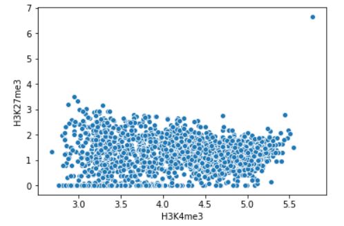
Fig. 3.27 Scatterplot (log-scale) between H3K4me3 and H3K27me3 within H3K4me3 peaks.
The command below draws a pairplot among all samples.
import numpy as np
import pandas as pd
import seaborn as sns

df = pd.read_csv("drompa.MULTICI.averaged.ChIPread.tsv",
                 sep="\t",
                 index_col=["chromosome","start","end"])
logdf = np.log1p(df)
g = sns.PairGrid(logdf)
g.map_upper(sns.scatterplot)
g.map_diag(sns.distplot)
g.map_lower(sns.kdeplot)
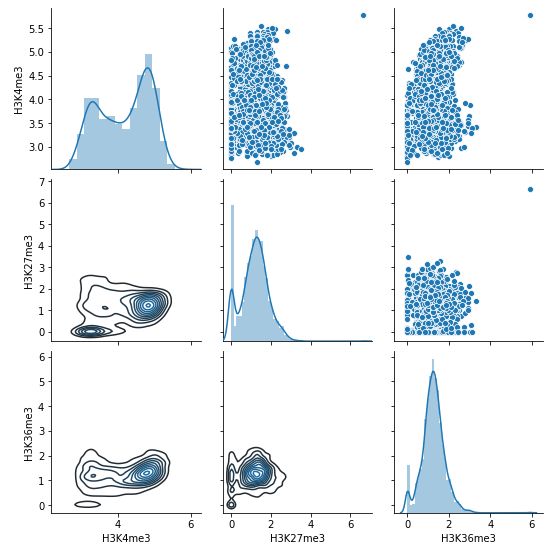
Fig. 3.28 Pairplot (log-scale) among three samples within H3K4me3 peaks.